Plotting in CP2KData

Color blind friendly colormaps

If a submitted manuscript happens to go to three male reviewers of Northern European descent, the chance that at least one will be color blind is 22 percent.

by [Won10]

This shows the importance of creating color blind friendly plots. As suggested by the above reference, I implemented the recommended color blind friendly colormaps in the CP2KData package. The usage is summarized in the following,

1. Register the colormaps using cp2kdata

   import matplotlib as mpl
   import cp2kdata.plots.colormaps
   

   #output
   color blind friendly colormap registered as cp2kdata_cb_lcmap
   color blind friendly colormap registered as cp2kdata_cb_lscmap
   

2. Get the colormaps

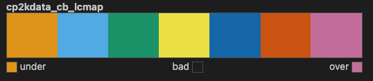
   There are two colormaps in the package. The first one is a listed colormap, which can also be understood as a discrete colormap.

   mpl.colormaps['cp2kdata_cb_lcmap']
   

   

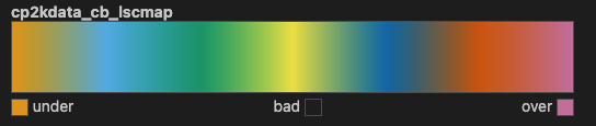
   The second one is a linear segmented colormap, which can also be understood as a continuous colormap.

   mpl.colormaps['cp2kdata_cb_lscmap']
   

   

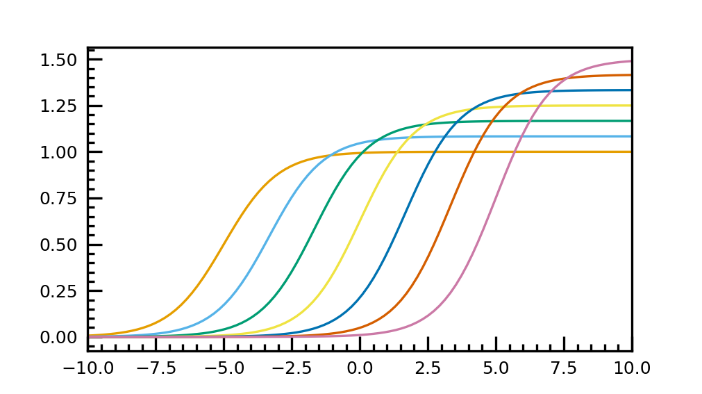
3. Example for using the listed colormap

   import matplotlib.pyplot as plt
   import matplotlib as mpl
   import numpy as np
   import cp2kdata.plots.colormaps
   plt.style.use('cp2kdata.matplotlibstyle.jcp')
   
   
   cp2kdata_cb_lcmap = mpl.colormaps['cp2kdata_cb_lcmap']
   plt.rcParams["axes.prop_cycle"] = plt.cycler("color", cp2kdata_cb_lcmap.colors)
   row = 1
   col = 1
   fig = plt.figure(figsize=(3.37*col, 1.89*row), dpi=300, facecolor='white')
   gs = fig.add_gridspec(row,col)
   ax  = fig.add_subplot(gs[0])
   
   t = np.linspace(-10, 10, 100)
   def sigmoid(t, t0):
       return 1 / (1 + np.exp(-(t - t0)))
   
   nb_colors = len(plt.rcParams['axes.prop_cycle'])
   
   shifts = np.linspace(-5, 5, nb_colors)
   amplitudes = np.linspace(1, 1.5, nb_colors)
   for t0, a in zip(shifts, amplitudes):
       ax.plot(t, a * sigmoid(t, t0), '-')
   ax.set_xlim(-10, 10)
   
   fig.savefig("cb_lcmap_plot.png", dpi=100)
   

   

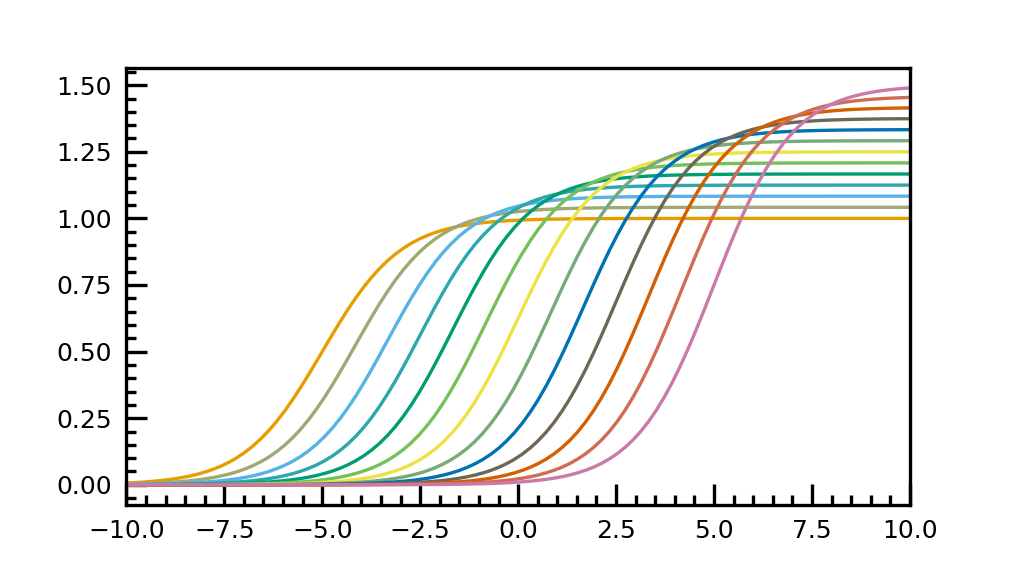
4. Example for using the linear segmented colormap

   import matplotlib.pyplot as plt
   import matplotlib as mpl
   import numpy as np
   import cp2kdata.plots.colormaps
   plt.style.use('cp2kdata.matplotlibstyle.jcp')
   
   
   cp2kdata_cb_lscmap = mpl.colormaps['cp2kdata_cb_lscmap']
   N = 13
   plt.rcParams["axes.prop_cycle"] = plt.cycler("color", cp2kdata_cb_lscmap(np.linspace(0,1,N)))
   row = 1
   col = 1
   fig = plt.figure(figsize=(3.37*col, 1.89*row), dpi=300, facecolor='white')
   gs = fig.add_gridspec(row,col)
   ax  = fig.add_subplot(gs[0])
   
   t = np.linspace(-10, 10, 100)
   def sigmoid(t, t0):
       return 1 / (1 + np.exp(-(t - t0)))
   
   nb_colors = len(plt.rcParams['axes.prop_cycle'])
   
   shifts = np.linspace(-5, 5, nb_colors)
   amplitudes = np.linspace(1, 1.5, nb_colors)
   for t0, a in zip(shifts, amplitudes):
       ax.plot(t, a * sigmoid(t, t0), '-')
   ax.set_xlim(-10, 10)
   
   fig.savefig("cb_lscmap_plot.png", dpi=100)
   

   

Other color blind friendly colormaps

One of the common used colormaps is viridis. We can find it in the seaborn package.

fig = plt.figure(figsize=(3.37*scale*col, 1.89*scale*row), dpi=300)
fig.subplots_adjust(hspace=0.3)
gs = fig.add_gridspec(row,col)


# read the averaged FES
file_fes =  f'fes-ave.dat'
bin_cn = 101
bin_d = 101
X = np.loadtxt(file_fes, usecols=0)
Y = np.loadtxt(file_fes, usecols=1)
Z = np.loadtxt(file_fes, usecols=2)
Z_std = np.loadtxt(file_fes, usecols=3)
X = X.reshape(bin_cn, bin_d)
Y = Y.reshape(bin_cn, bin_d)
Z = Z.reshape(bin_cn, bin_d)
Z_std = Z_std.reshape(bin_cn, bin_d)
Z = Z*0.0103636  # to eV
Z_std = Z_std*0.0103636  # to eV
Z_min = np.min(Z)
Z = Z - Z_min

Z = Z.clip(min=vmin, max=vmax)

ax  = fig.add_subplot(gs[0])

my_cmp = sns.color_palette("viridis", as_cmap=True)
CS = ax.contour(X, Y, Z,levels=int(levels/4), vmin=vmin, vmax=vmax, colors='k', linewidths=0.4, labcex=10)
CS2 = ax.contourf(X,Y,Z,levels=levels, cmap=my_cmp.reversed(), vmin=vmin, vmax=vmax)

ax.clabel(CS, fontsize=6, inline=True, fmt="%1.2f")
ax.set_xlim(2.0, 4.5)
ax.set_ylim(0.6, 2.6)
ax.set_xlabel(r"X", fontsize=fontsize)
ax.set_ylabel(r"Y", fontsize=fontsize)
cbar = fig.colorbar(mappable=CS2, ax=ax)
cbar.set_label(r"Z", fontsize=fontsize)