Band alignment#
Introduction#
Usage#
from ectoolkits..analysis.band_align import BandAlign
inp = {
     "input_type": "cube",
     "ave_param":{
         "prefix": "./00.interface/hartree/Hematite-v_hartree-1_",
         "index": (1, 502),
         "l1": 4.8,
         "l2": 4.8,
         "ncov": 2,
         "save": True,
         "save_path":"00.interface"
     },
     "shift_param":{
         "surf1_idx": [124, 125, 126, 127, 128, 129, 130, 131],
         "surf2_idx": [24, 25, 26, 27, 28, 29, 30, 31]
     },
     "water_width_list": [8, 9, 9.5, 10, 10.5, 11, 12, 13],
     "solid_width_list": [1, 2, 3, 4]

}
ba = BandAlign(inp)
#quick view of hartree fluctuation
fig = ba.plot_hartree_per_width('water')
fig = ba.plot_hartree_per_width('solid')

# detail information is accessible in
ba.water_hartree_list
ba.solid_hartree_list
Prepare Input Data#
One has to collect all hartree cube files from continuous MD simulations in one directory with same prefix and suffix of .cube.
For example, in directory ./00.interface/hartree/, one should prepare cube file named Hematite-v_hartree-1_1.cube, Hematite-v_hartree-1_2.cube, …, Hematite-v_hartree-1_501.cube.
Explanation for Parameters#

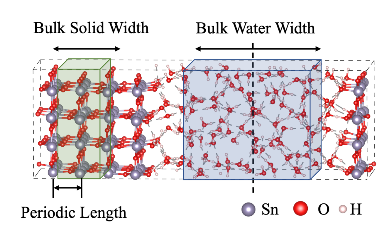
input_type:cubefor cp2k cube filesprefix: define prefix for cube filesindex: define the index for cube files, seePrepare Input Datal1: parameter for nanosmoothing.l1equals to natural number (n) times periodic length (pl) for oxides slab. For example, the z position of a layer for \(\mathrm{SnO_2}\)(110) slab is defined as the ensemble-averaged z positions of \(\mathrm{Sn}\) atoms in the layer. Then, the periodic length is inter-layer distance between two layers. Assumingplis 2.4 \(\mathrm{\AA}\),l1can be 2.4, 4.8, and 7.2 \(\mathrm{\AA}\).l2: parameter for nanosmoothing.l2equals to natural number (n) times periodic length (pl) for water. Since water dose not have periodicity, we recommend to setl2same asl1.ncov: parameter for nanosmoothing.ncovis number of convolution.ncovequals to 2 for interfaces and equals to 1 for surface (slab-vacuum). Whenncovis 1,l2won’t be used.save: whether to save post processed hartree data. We recommend to set it asTrue.save_path: save_path for post processed hartree data.surf1_idx:place holdersurf2_idx:place holderwater_width_list: Width for bulk water. Bulk Water Width is plotted in above figure. Since one has to test multiple width value, the width is input as a list.solid_width_list: Width for Bulk Solid. Bulk Solid Width is plotted in above figure. Since one has to test multiple width value, the width is input as a list.
Plot Band Alignment Data#
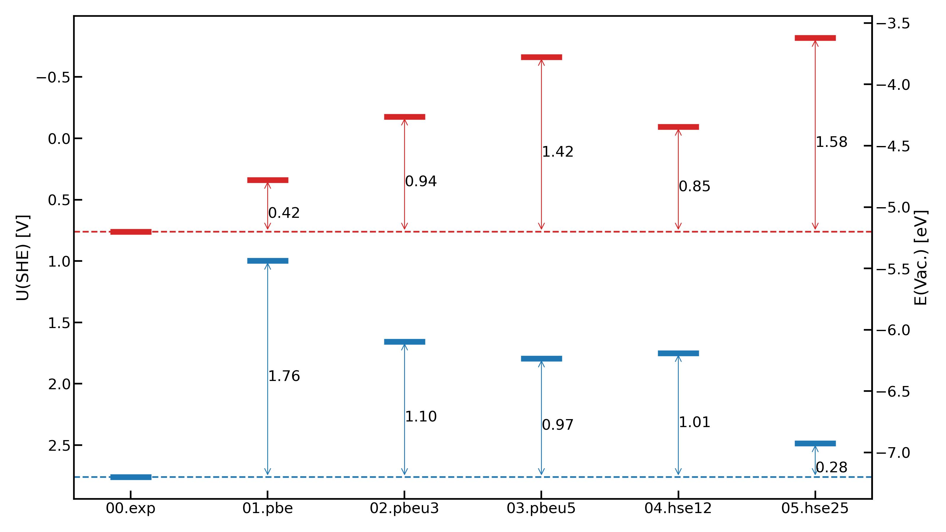
After Obtain band positions from post processing, you can plot these data using plot_band_alignment
from ectoolkits.plots.band_align import plot_band_alignment

#prepare your band positions data in dictionary format
ba_data = {
    "sys_1": {
        "vbm": 1.0,
        "cbm": -0.5
    },
    "sys_2": {
        "vbm": 1.2,
        "cbm": -0.3
    },
    ....
}
fig = plot_band_alignment(ba_dict=ba_data, show_diff=True, vac_value=False)
fig.savefig("bandalignment.png")
We assume the vbm and cbm values are in SHE scale. If the vbm and cbm values are referred to Vacuum scale, set vac_value=True. If you want to plot the difference between band position of first system and other systems, set show_diff=True.
